Computing Intracellular Distance Matrices
CAJAL represents a cell as a finite set of uniformly sampled points from its outline together with a notion of distance between each pair of points. This cell data is internally represented as an intracellular distance matrix, where each rows and column corresponds to a point in the cell, and the entry at position (i, j) denotes the distance between points x_i and x_j. Typically, 50 to 200 sampled points per cell are sufficient for most applications.
To compute the Gromov-Wasserstein distance between two cells, users need to first convert their cell morphology data into intracellular distance matrices. In this regard, CAJAL offers functionality that supports three kinds of input data files neuronal tracing data (SWC files), 3D meshes (OBJ files), and 2D cell segmentation files (TIFF files). This section describes how to leverage this functionality to produce intracellular distance matrices that enable users to perform Gromov-Wasserstein distance computations.
Euclidean vs. geodesic distances
CAJAL supports two types of intracellular distances matrices: Euclidean distance, which is the ordinary straight-line distance through the ambient space, and geodesic distance, which is the length of the shortest path through the surface of the cell. The choice between using Euclidean or geodesic distance affects the types of deformations that CAJAL considers relevant when comparing the shape of two cells.
Using Euclidean distance to measure intracellular distances results in morphological distances that are insensitive to translations, rotations, or mirroring of a cell. However, bending or flexing a cell will change the morphological distance between that cell and other cells. On the other hand, using geodesic intracellular distances leads to morphological distances that are insensitive to translations, rotations, mirroring, bending, and flexing of the cells.
To illustrate the distinction, consider two pieces of string, A and B, both of which are twelve inches long. If A is laid out in a straight line and B is tightly coiled, then the Gromov-Wasserstein distance between them will be nontrivial in they are represented by Euclidean intracellular distance matrices. This is because one must bend B to straighten it out into a line segment. However, if they are represented by their geodesic distance matrices, then the Gromov-Wasserstein distance will be zero. This is because one can deform A into B without any stretching or elongating, as they are the same length.
Neuronal Tracing Data
CAJAL supports neuronal tracing data in the SWC specification defined here.
You can find examples of *.swc files compatible with CAJAL can be found in the CAJAL Github
repository under CAJAL/data/swc_files.
The package provides two functions that operate on directories of *.swc files.
cajal.sample_swc.compute_icdm_all_euclidean() and cajal.sample_swc.compute_icdm_all_geodesic(). These functions
generate intracellular distance matrices for each cell in the source directory
and populate a *.csv file with the results.
For example, if you have a directory called /home/jovyan/CAJAL/CAJAL/data/swc_files that contains *.swc files and you want to write the intracellular distance matrices to a *.csv file called /home/jovyan/CAJAL/CAJAL/data/swc_icdm.csv, you can use the following code.
failed_cells = sample_swc.compute_icdm_all_euclidean(
    infolder = "/home/jovyan/CAJAL/CAJAL/data/swc_files",
    out_csv= "/home/jovyan/CAJAL/CAJAL/data/swc_icdm.csv",
    n_sample = 50,
    preprocess=swc.preprocessor_eu(
        structure_ids=[1,3,4],
        soma_component_only=True),
    num_processes = 8
    )
The n_sample argument specifies the number of points from each cell that will be sampled (we recommend between 50-100). The num_processes argument specifies the number of processes that will be launched in parallel, and we recommend setting it to the number of cores on your machine.
The preprocess argument is optional and can be used to filter out some neurons from being sampled, for reasons of data quality, and/or transform the remaining data before sampling from it. The argument is very flexible and can be used in many ways. For convenience, two specific use cases are built-in. The line structure_ids = [1,3,4] indicates that samples will only be drawn from the node types corresponding to 1, 3 and 4 in the SWC specification, i.e., the soma and basal and apical dendrites. This can be useful when the user has a mixture of full neuronal reconstructions and dendrite-only neuronal reconstructions and wants to discard the axons from the full neuronal reconstructions. To keep all node types, set structure_ids = “keep_all_types”. The argument soma_component_only=True indicates that the function will only sample from the unique component of the neuron containing the soma, and will write to an error log any neurons which do not contain a unique component containing nodes labeled as soma. This illustrates the basic function of the preprocessing function, in this example filtering out all neurons which don’t have a unique soma node, and transforming the remaining neurons by discarding all components except the one containing the unique soma node. To keep all connected components, set soma_component_only=False.
The function returns a list called failed_cells that contains the names of the cells for which sampling was unsuccessful (i.e., the preprocessing function returned an error) together with the error itself. If the sampling is successful, the results are silently written to a file.
A similar functionality is implemented in cajal.sample_swc.compute_icdm_all_geodesic()
with respect to the computation of intracellular geodesic distances.
3D meshes
CAJAL provides support for Wavefront *.obj 3D mesh files. The package expects each line of a mesh file to be one of the following.
A comment, marked with a “#”
A vertex, written as v float1 float2 float3
A face, written as f linenum1 linenum2 linenum3
Examples of *.obj files compatible with CAJAL can be found in the CAJAL Github
repository under the folder CAJAL/data/obj_files.
It is important to note that a *.obj file may contain several distinct connected components. By default, CAJAL separates these components into individual cells. However, in situations where a *.obj file is supposed to represent a single cell but has multiple disconnected components due to measurement errors, the package provides functionality to create a new mesh where all components are joined together by new faces. This allows for the computation of a geodesic distance between points in the mesh. If the user wants to compute the Euclidean distance between points, such repairs are unnecessary, as the Euclidean distance is insensitive to connectivity.
CAJAL provides one batch-processing function that goes through all *.obj files in a given directory, separates them into connected components, computes intracellular distance matrices for each component, and writes all these square matrices to a *.csv file. For example,
failed_samples = sample_mesh.compute_icdm_all(
            infolder="/home/jovyan/CAJAL/data/obj_files",
            out_csv="/home/jovyan/CAJAL/data/sampled_pts/obj_geodesic_50.csv",
            metric = "segment",
            n_sample=50,
            num_cores=8,
            segment = True,
            method="heat"
            )
The arguments infolder, out_csv, n_sample, metric are as in Neuronal Tracing Data, except that infolder is a folder containing *.obj files rather than *.swc files.
If the Boolean flag segment is True, the function will break down each *.obj file into its connected components and treat them as individual, isolated cells. If segment is set to False, the function will treat each *.obj file as a single cell. If the user chooses the “geodesic” metric and the contents of a *.obj file are not connected, CAJAL will automatically attempt to “repair” the cell by modifying it to adjoin new paths between connected components, so that a geodesic distance between points can be defined.
Warning
Modifying the data by adjoining new triangles to the mesh is an imputation of data which changes its topology. This presents the same thorny questions as in any other scenario when data is imputed, and the user should keep this in mind while interpreting the data. The functionality of “repairing” the cell is premised on the assumption that the *.obj file represents a single geometric object and that it fails to be connected for trivial reasons. If a *.obj file genuinely contains multiple distinct components, then the geodesic distances resulting from this process will not be meaningful.
Segmentation files
Image segmentation is the process of separating an image into distinct components to simplify the representations of objects. Morphological segmentation is one approach to image segmentation based on morphology. While CAJAL provides tools to sample from the cell boundaries of segmented image files, it is important to note that CAJAL is not a tool for image segmentation itself. Users are expected to segment and clean their own images.
To help users prepare their data for use with CAJAL, we provide a basic example
using images from the CAJAL Github repository (CAJAL/data/tiff_images).
Let us consider the following image
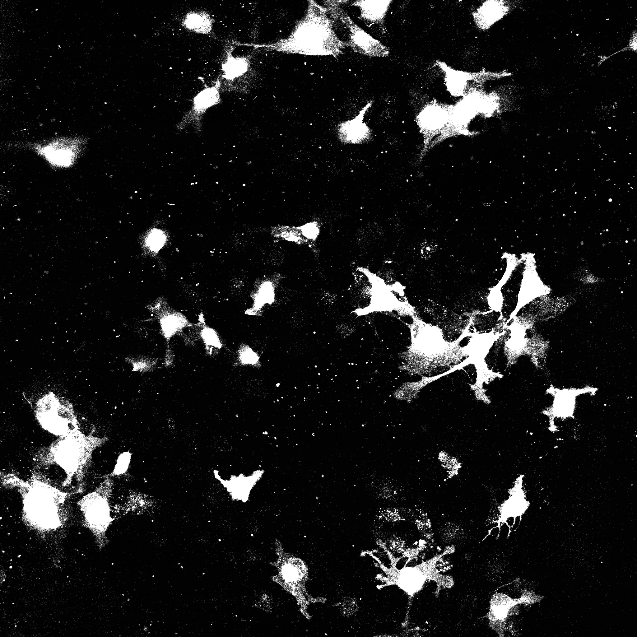
The OpenCV package provides some basic functionality to clean image data and
perform segmentation. Users can use the cv.imread() function to load *.tiff
files into memory.
import tifffile

img=tifffile.imread(CAJAL/data/tiff_images/epd210cmd1l3_1.tif)
We then recommend collapsing the greyscale image to black and white and performing dilation followed by erosion and erosion followed by dilation to remove noise and small holes.
import cv2 as cv
import numpy as np

_, thresh = cv.threshold(img,100,255,cv.THRESH_BINARY)
kernel = np.ones((5,5),np.uint8)
closing = cv.morphologyEx(thresh, cv.MORPH_CLOSE, kernel)
closethenopen = cv.morphologyEx(closing, cv.MORPH_OPEN,kernel)
Afterward, users can label each connected region of the image with a unique common color.
from skimage import measure

labeled_img = measure.label(closethenopen)
The image is still somewhat noisy, with a few specks in it. To despeckle it, we can remove all connected regions with fewer than 1000 pixels by grouping them into the background region, which is labelled with 0.
labels = np.unique(labeled_img, return_counts=True)
labels = (labels[0][1:],labels[1][1:])
remove = np.isin(labeled_img, labels[0][labels[1]<1000])
img_keep = labeled_img.astype(np.uint8)
img_keep[remove] = 0
We can use matplotlib to view the image from an interactive environment like Jupyter notebook.
import matplotlib.pyplot as plt
fig, ax = plt.subplots()
ax.imshow(simplify_img_keep)
fig.set_size_inches(30, 30)
plt.show()
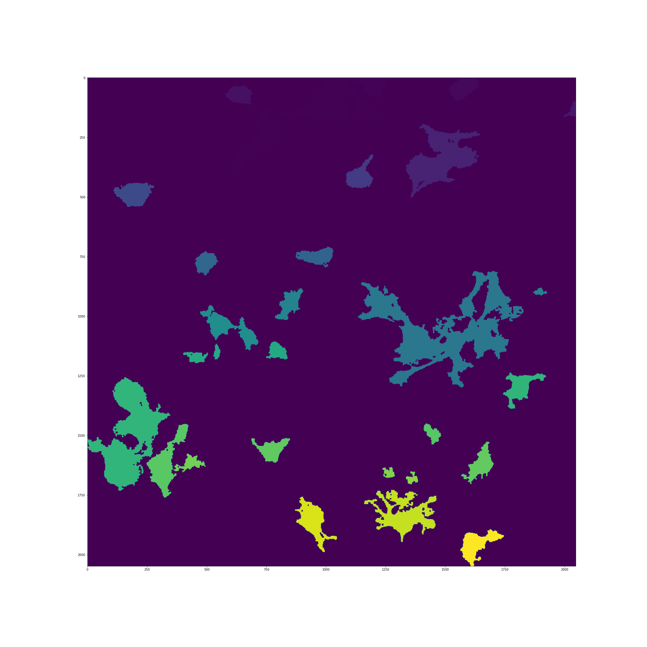
This image is representative of the type of images that CAJAL is meant to process: a 2D array of integers, where each cell is represented by a connected block of integers with the same value. Two distinct cells should have different values, and each cell should have a different value than the background.
We can write the cleaned image to a file using tifffile.imwrite().
tifffile.imwrite('/home/jovyan/CAJAL/CAJAL/data/cleaned_file.tif',
img_keep, photometric='minisblack')
It is essential to note that this is only a toy example. For instance, in this image multiple overlapping cells have been grouped into a single mask. Users would normally discard such overlapping cells before analysis with CAJAL.
To sample points and compute intracellular distances from *.tiff / *.tif files
like these, CAJAL provides the function
cajal.sample_seg.compute_icdm_all(). This function takes
an input directory full of cleaned *.tiff/*.tif files and an output
directory as arguments. For each *.tiff file in the input directory,
cajal.sample_seg.compute_icdm_all() breaks the image down into
its separate cells, samples a given number of points for each one, and
writes the resulting resulting intracellular distance matrix for each cell to a
single collective database for all files in the directory.
infolder ="/home/jovyan/CAJAL/CAJAL/data/tiff_images_cleaned/"
out_csv="/home/jovyan/CAJAL/CAJAL/data/tiff_sampled_50.csv"
sample_seg.compute_icdm_all(
               infolder,
               out_csv,
               n_sample = 50,
               num_cores = 8,
               background = 0,
               discard_cells_with_holes = False,
               only_longest = False
               )
infolder specifies the input directory of cleaned *.tiff/*.tif files, db_name indicates the name of the database file, and n_sample the number of points to sample from each cell. background is the index for the background color, which is 0 by default. If the flag discard_cells_with_holes is set to True, the function will ignore any cells that have multiple boundaries. The argument only_longest is only relevant if discard_cells_with_holes is False. In this case if only_longest is True, then the function only samples from the longest boundary of the cell instead of across all boundaries. Cells that meet the image boundary are discarded.