Tutorial 1: Predicting the Molecular Type of Neurons
To demonstrate some of the main functionalities of CAJAL, here we perform some basic analysis on a set of neuron morphological reconstructions obtained from the Allen Brain Atlas. To facilitate the analysis, we provide a compressed *.tar.gz file containing the *.SWC files of 509 neurons used in this example, which can be downloaded directly from this
link. In this tutorial we assume that the SWC files are located in the folder /home/jovyan/swc. More information about this dataset can be found at:
Gouwens, N. W. et al. Classification of electrophysiological and morphological neuron types in the mouse visual cortex. Nat Neurosci 22, 1182-1195 (2019).
For this analysis, we focus on the morphology of the dendrites and exclude the axons of the neurons. To achieve this, we set structure_ids = [1,3,4], which tells CAJAL to only sample points from the soma and the basal and apical dendrites. We sample 100 points from each neuron and compute the Euclidean distance between each pair of points in that neuron using the following code:
[1]:
import cajal.sample_swc
import cajal.swc
from os.path import join
[2]:
bd = "/home/jovyan/" # Base directory
[3]:
cajal.sample_swc.compute_icdm_all_euclidean(
    infolder=join(bd, 'swc'),
    out_csv=join(bd, 'swc_bdad_100pts_euclidean_icdm.csv'),
    out_node_types=join(bd, 'swc_bdad_100pts_euclidean_node_types.npy'),
    preprocess=cajal.swc.preprocessor_eu(
        structure_ids=[1,3,4],
        soma_component_only=False),
    n_sample=100)
100%|█████████▉| 508/509 [00:23<00:00, 21.23it/s]
[3]:
[]
Once the sampling is completed, we compute the Gromov-Wasserstein distance between each pair of neurons. To compute the Gromov-Wasserstein distance matrix we use the code:
[5]:
import cajal.run_gw

cajal.run_gw.compute_gw_distance_matrix(
    join(bd, 'swc_bdad_100pts_euclidean_icdm.csv'),
    join(bd, 'swc_bdad_100pts_euclidean_GW_dmat.csv'),
    gw_coupling_mat_npz_loc=join(bd, 'swc_bdad_100pts_euclidean_GW_couplings.npz'),
    num_processes=15)
[5]:
(array([[ 0.        , 48.00771782, 23.044745  , ..., 31.6661131 ,
         28.23034998, 15.52264516],
        [48.00771782,  0.        , 58.39010605, ..., 68.06746526,
         66.14810561, 55.62932524],
        [23.044745  , 58.39010605,  0.        , ..., 19.22607515,
         19.66919727, 23.99896955],
        ...,
        [31.6661131 , 68.06746526, 19.22607515, ...,  0.        ,
         10.71261723, 30.50133611],
        [28.23034998, 66.14810561, 19.66919727, ..., 10.71261723,
          0.        , 29.15049728],
        [15.52264516, 55.62932524, 23.99896955, ..., 30.50133611,
         29.15049728,  0.        ]]),
 None)
We can visualize the resulting space of cell morphologies using UMAP:
[4]:
import plotly.io as pio

# Choose the adequate plotly renderer for visualizing plotly graphs in your system
pio.renderers.default = 'notebook_connected'
# pio.renderers.default = 'iframe'

import cajal.utilities
from umap import umap_
import plotly.express

# Read GW distance matrix
cells, gw_dist_dict = cajal.utilities.read_gw_dists(join(bd,"swc_bdad_100pts_euclidean_GW_dmat.csv"), header=True)
gw_dist = cajal.utilities.dist_mat_of_dict(gw_dist_dict, cells)

# Compute UMAP representation
reducer = umap_.UMAP(metric="precomputed", random_state=1)
embedding = reducer.fit_transform(gw_dist)

# Visualize UMAP
plotly.express.scatter(x=embedding[:,0],
                       y=embedding[:,1],
                       template="simple_white",
                       hover_name=[m + ".swc" for m in cells])
/home/patn/PGC012_Gromov_Wasserstein/venv/lib/python3.12/site-packages/umap/umap_.py:1780: UserWarning:

using precomputed metric; inverse_transform will be unavailable
Once the user has computed the Gromov-Wasserstein distances between cells it is possible to cluster the cells using standard clustering techniques. The Louvain and Leiden clustering algorithms are two commonly used algorithms to identify communities within large networks; they can be adapted to finite metric spaces by constructing a k-nearest-neighbors graph on top of the metric space. CAJAL provides access to both of these clustering algorithms. When combined with a low-dimensional embedding tool such as the UMAP algorithm, the user can plot the clusters in a 2-dimensional embedding and visualize them. Here, we use the Leiden algorithm to cluster the neurons based on their morphology:
[5]:
clusters = cajal.utilities.leiden_clustering(gw_dist, seed=1)
plotly.express.scatter(x=embedding[:,0],
                       y=embedding[:,1],
                       template="simple_white",
                       hover_name=[m + ".swc" for m in cells],
                       color = [str(m) for m in clusters])
/home/patn/PGC012_Gromov_Wasserstein/venv/lib/python3.12/site-packages/plotly/express/_core.py:1992: FutureWarning:

When grouping with a length-1 list-like, you will need to pass a length-1 tuple to get_group in a future version of pandas. Pass `(name,)` instead of `name` to silence this warning.
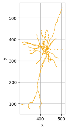
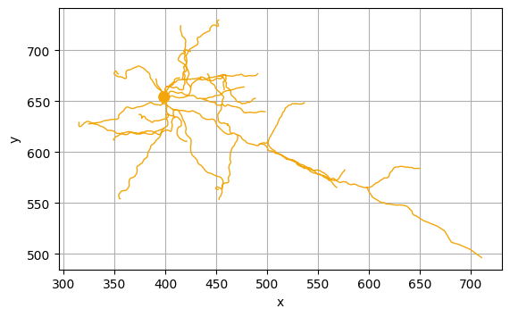
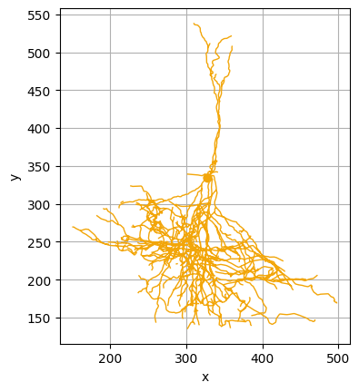
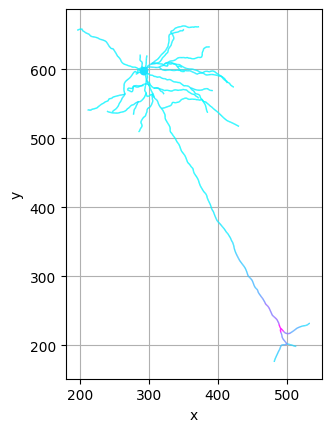
As expected, cells belonging to the same cluster have similar morphology. For example, let us visualize some of the cells in the brown cluster (cluster 8) using the Python package NAVis (which can be installed using pip install navis):
[6]:
import navis

cells_cluster_8 = [n for m, n in zip(clusters, cells) if m==8]
cluster_8 = [navis.read_swc(join(bd,"swc/" + n + ".swc")) for n in cells_cluster_8]

cluster_8[1].plot2d()
cluster_8[2].plot2d()
cluster_8[3].plot2d()
[6]:
(<Figure size 640x480 with 1 Axes>, <Axes: xlabel='x', ylabel='y'>)
NAVis offers many other great functionalities, including interactive 3D visualizations of the neurons using plot3d(). More information about those functionalities can be found at the NAVis documentation.
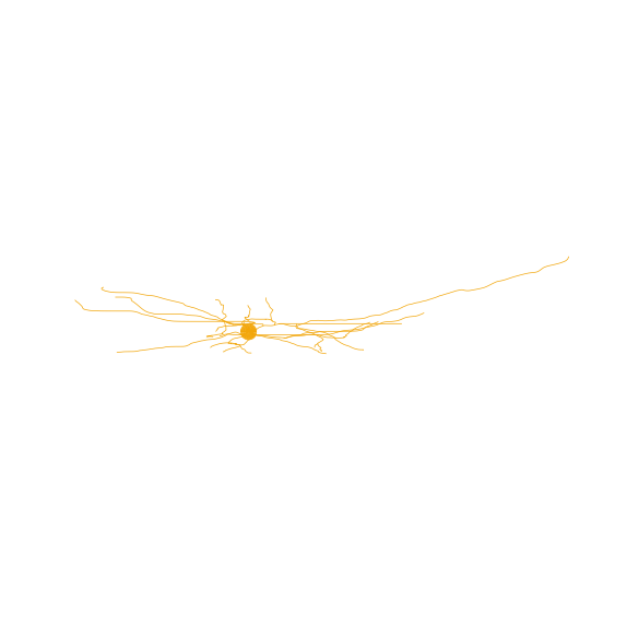
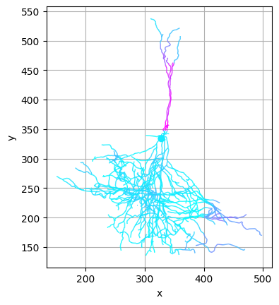
We can also compute the medoid of the cluster, i. e. the most central neuron of the cluster (and therefore a good representative of the morphologies present in the cluster), and visualize it:
[7]:
medoid_8 = navis.read_swc(join(bd,'swc/' + cajal.utilities.identify_medoid(cells_cluster_8, gw_dist_dict) + ".swc"))
medoid_8.plot2d()
[7]:
(<Figure size 640x480 with 1 Axes>, <Axes: xlabel='x', ylabel='y'>)
CAJAL allows the user to visualize the components of each neuron which contribute the most to the overall morphological distance. Here, we compare the medoid neurons of the 5th and 8th clusters. Regions in red represent morphological distinctions between the two cells.
[8]:
from cajal.deformation_vis import navis_heatmap

cells_cluster_5 = [n for m, n in zip(clusters, cells) if m==5]
medoid_5 = navis.read_swc(join(bd,'swc/' + cajal.utilities.identify_medoid(cells_cluster_5, gw_dist_dict) + ".swc"))
(heatmap_5, heatmap_8) = navis_heatmap(medoid_5, 200, medoid_8, 200)
[9]:
heatmap_5.plot2d(color_by='distortion', palette='cool')
heatmap_8.plot2d(color_by='distortion', palette='cool')
[9]:
(<Figure size 640x480 with 1 Axes>, <Axes: xlabel='x', ylabel='y'>)
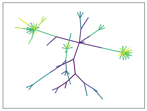
Another tool CAJAL offers to better understand the morphological characteristics of a cluster of cells is an “average spanning tree” algorithm, which takes as input a cluster of morphologically similar neurons and returns a topological tree structure which is representative of the topology and branching characteristics of cells in the cluster; visualizing this tree can give intuition into the basic commonalities in the cluster.
The concept behind the algorithm is that, since the Gromov-Wasserstein distance offers a way to align cells with each other, after identifying the medoid cell of the cluster, we can align the cells with the medoid cell using the optimal transport plans, which makes it possible to superimpose the graphs in a meaningful way and take the arithmetic average of their adjacency matrices.
The graph can be visualized with any standard Python graph library, such as Networkx. We illustrate the usage here with the computation of the average spanning tree for cells in cluster 0,
[10]:
gw_coupling_mat_dict=cajal.utilities.read_gw_couplings(join(bd, 'swc_bdad_100pts_euclidean_GW_couplings.npz'))
cell_icdms = dict(cajal.utilities.cell_iterator_csv(
    join(bd, 'swc_bdad_100pts_euclidean_icdm.csv'),
    as_squareform=False)
    )

def plot_graph(adjacency_matrix, confidence):
    import networkx as nx
    import matplotlib.pyplot as plt
    import numpy as np
    G=nx.Graph(adjacency_matrix, confidence=confidence)
    pos = nx.spring_layout(G)
    color = np.arange(len(G.nodes))
    plot_color = color[[i[1] for i in G.edges]]
    _, ax = plt.subplots()
    nx.draw_networkx_edges(G, pos, alpha=1, width=2, ax=ax, edge_color=plot_color)
    nx.draw_networkx_nodes(G, pos, nodelist=G.nodes, node_color=color, node_size=2, ax=ax)
    plt.show()

(adjacency_matrix, confidence) = cajal.utilities.avg_shape_spt(
    [n for m, n in zip(clusters, cells) if m==0],
    gw_dist_dict,
    cell_icdms,
    gw_coupling_mat_dict,
    k=3)

plot_graph(adjacency_matrix, confidence)
/tmp/ipykernel_46323/734124012.py:16: DeprecationWarning:

`alltrue` is deprecated as of NumPy 1.25.0, and will be removed in NumPy 2.0. Please use `all` instead.
Let us now study the association of other neuronal features with the morphology of the neurons. The file CAJAL/data/cell_types_specimen_details.csv in the GitHub repository of CAJAL contains metadata for each of the neurons in this example, including the layer, Cre line, etc. Here we color the above UMAP representation by the cortical layer of each neuron:
[11]:
import pandas

metadata = pandas.read_csv(join(bd,"cell_types_specimen_details.csv"))
metadata.index = [str(m) for m in metadata["specimen__id"]]
metadata = metadata.loc[cells]

plotly.express.scatter(x=embedding[:,0],
                       y=embedding[:,1],
                       template="simple_white",
                       hover_name=[m + ".swc" for m in cells],
                       color = metadata["structure__layer"])
/home/patn/PGC012_Gromov_Wasserstein/venv/lib/python3.12/site-packages/plotly/express/_core.py:1992: FutureWarning:

When grouping with a length-1 list-like, you will need to pass a length-1 tuple to get_group in a future version of pandas. Pass `(name,)` instead of `name` to silence this warning.
As shown in the visualization, different cortical layers seem to be associated with specific regions of the cell morphology space. We can quantify statistically the association using the Laplacian score:
[12]:
import cajal.laplacian_score
import numpy
import pandas
from scipy.spatial.distance import squareform

# Build indicator matrix
layers = numpy.unique(metadata["structure__layer"])
indicator = (numpy.array(metadata["structure__layer"])[:,None] == layers)*1

# Compute the Laplacian score
laplacian = pandas.DataFrame(cajal.laplacian_score.laplacian_scores(indicator,
                                       gw_dist,
                                       numpy.median(squareform(gw_dist)),
                                       permutations = 5000,
                                       covariates = None,
                                       return_random_laplacians = False)[0])
laplacian.index = layers

print(laplacian)
     feature_laplacians  laplacian_p_values  laplacian_q_values
1              0.976417              0.0004            0.000600
2/3            0.968974              0.0002            0.000600
4              0.969925              0.0002            0.000600
5              0.987595              0.0002            0.000600
6a             0.992887              0.0022            0.002639
6b             0.992448              0.0024            0.002400
We observe that indeed all cortical layers are significantly associated with distinct regions of the cell morphology space, with false discovery rates (FDRs) < 0.05.
We could perform a similar analysis with other features. Alternatively, we could build a classifier to predict the value of each feature based on the position of the cells in the cell morphology space. For example, each neuron in the dataset is derived from a specific Cre driver line, which preferentially labels distinct neuronal types. Neurons from the same Cre driver line therefore tend to have similar morphologies, and a Laplacian score analysis would show that many Cre driver lines are significantly associated with distinct regions of the cell morphology space. As a result, it is possible to predict the Cre driver line of a neuron based on its morphological features.
To accomplish this, we train a nearest-neighbors classifier on the GW distance matrix and evaluate its accuracy using 7-fold cross-validation:
[13]:
from sklearn.neighbors import KNeighborsClassifier
from sklearn.model_selection import StratifiedKFold, cross_val_score

cre_lines = numpy.array(metadata["line_name"])

clf = KNeighborsClassifier(metric="precomputed", n_neighbors=10, weights="distance")
cv = StratifiedKFold(n_splits=7, shuffle=True,random_state=0)
accuracy = cross_val_score(clf, X=gw_dist, y=cre_lines,cv=cv)

numpy.mean(accuracy)
/home/patn/PGC012_Gromov_Wasserstein/venv/lib/python3.12/site-packages/sklearn/model_selection/_split.py:776: UserWarning:

The least populated class in y has only 1 members, which is less than n_splits=7.
[13]:
0.2964231354642313
Similarly, we can compute the Matthews correlation coefficient of the classification, which appropriately weights the error arising from misclassifying elements of smaller classes:
[14]:
from sklearn.model_selection import cross_val_predict
from sklearn.metrics import matthews_corrcoef

cvp = cross_val_predict(clf, X=gw_dist, y=cre_lines, cv=cv)

print(matthews_corrcoef(cvp, cre_lines))
0.24254759274161383
/home/patn/PGC012_Gromov_Wasserstein/venv/lib/python3.12/site-packages/sklearn/model_selection/_split.py:776: UserWarning:

The least populated class in y has only 1 members, which is less than n_splits=7.