Tutorial 6: Morphology-Aware Analysis of Subcellular Protein Localization (CellAligner)
To demonstrate the functionality of CellAligner-OT, this tutorial analyzes 2D immunofluorescence images from the Human Protein Atlas. We will use a small subset of 373 cells from 70 images, available for download here.
[ ]:
import os
import pandas as pd
import matplotlib.pyplot as plt
from tqdm import tqdm
import skimage as ski
from cajal.subcellular import *

# change to path to where data is located
data_path = '/workspaces/CellAligner/hpa_images_metadata/'

# load image metadata
image_metadata = pd.read_csv(os.path.join(data_path, 'image_metadata.csv'), index_col=0)
We begin by processing the cell images by sampling points from the cell boundary for morphological analysis and extracting information needed for localization analysis. We assume that cell segmentation has already been performed for each image. Nuclear segmentation is optional, but can substantilly improve localization analysis.
[3]:
# create list to store cell objects
cell_objects = []
cell_metadata = pd.DataFrame(columns=image_metadata.columns)
for i in tqdm(range(image_metadata.shape[0])):
    im_path = os.path.join(data_path, 'images', image_metadata.iloc[i]['image_file'])
    # load image
    im = ski.io.imread(im_path)
    channels = ['microtubules', 'protein', 'DNA'] # names of channels in image
    # load cell and nuclear segmentation masks
    im_cell_mask = ski.io.imread(im_path.replace('blue_red_green.jpg','predictedmask.png'))
    im_nuc_mask = ski.io.imread(im_path.replace('blue_red_green.jpg','predictednucmask.png'))
    # create cell objects from image
    image_cell_objects = process_image(im, channels, im_cell_mask, im_nuc_mask, ds_target_size=1000)
    cell_objects.extend(image_cell_objects)
    # save metadata for each cell
    n_image_cells = len(image_cell_objects)
    cell_metadata = pd.concat([cell_metadata, image_metadata.iloc[i:i+1].reset_index(drop=True).loc[np.repeat(0, n_image_cells)]], ignore_index=True)
100%|██████████| 60/60 [06:32<00:00, 6.54s/it]
The resulting CellAligner_Cell objects can be kept in memory for faster analysis or written to disk when memory is limited. All functions that take CellAligner_Cell objects as input also accept paths to saved CellAligner_Cell objects.
To quantify morphological variation across cells, we compute the Gromov-Wasserstein distance between each pair of cells based on points sampled from their boundaries using intracellular Euclidean distances.
[4]:
gw_dmat = gw_pairwise_parallel(cell_objects, num_processes=cpu_count(), chunksize=20)
100%|██████████| 69378/69378 [31:22<00:00, 36.86it/s]
We can then cluster cells based on their pairwise Gromov-Wasserstein morphology distances to identify groups with similar morphologies. For visualization, we can use UMAP to embed the morphology space in two dimensions.
[6]:
import plotly.io as pio

# Choose the adequate plotly renderer for visualizing plotly graphs in your system
pio.renderers.default = 'notebook_connected'
# pio.renderers.default = 'iframe'

import cajal.utilities
import umap
import plotly.express

# Compute UMAP representation of the GW morphology space
reducer = umap.UMAP(metric="precomputed", random_state=1)
embedding = reducer.fit_transform(gw_dmat)

# Cluster cells based on the GW morphology space using the leiden algorithm
gw_clusters = cajal.utilities.leiden_clustering(gw_dmat, resolution=0.003, seed=1)

# Visualize the GW morphology space
plotly.express.scatter(x=embedding[:,0],
                       y=embedding[:,1],
                       template="simple_white",
                       hover_name=["cell_" + str(i) for i in range(gw_dmat.shape[0])],
                       color = [str(c) for c in gw_clusters]
                       )
/opt/conda/lib/python3.12/site-packages/umap/umap_.py:1865: UserWarning:

using precomputed metric; inverse_transform will be unavailable

/opt/conda/lib/python3.12/site-packages/umap/umap_.py:1952: UserWarning:

n_jobs value 1 overridden to 1 by setting random_state. Use no seed for parallelism.
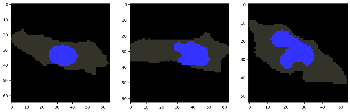
Cells within the same cluster are expected to have similar morphologies. For example, we can visualize several cells from cluster 1.
[7]:
cells_to_plot = [122, 177, 188] # Example cells from cluster 1
fig, axes = plt.subplots(1, len(cells_to_plot), figsize=(15, 5))
for ax, i in zip(axes, cells_to_plot):
    plot_cell_image(cell_objects[i], channels=['nucleus'], ax=ax)
plt.show()
Before quantifying variation in subcellular localization patterns, we first map the protein localization pattern of each cell to an anchor cell. We recommend choosing the centroid cell in the morphology space as the anchor.
There are two approaches for mapping cells to the anchor: Fused Gromov-Wasserstein and Fused Unbalanced Gromov-Wasserstein. Fused Gromov-Wasserstein performs a full cell-to-cell mapping, which is appropriate for datasets with relatively simple cell morphologies. Fused Unbalanced Gromov-Wasserstein allows partial cell-to-cell mappings, which is useful for datasets with more complex cell morphologies, such as neurons, where certain cellular structures may be present in one cell but absent in another.
The “fused” variant of Gromov-Wasserstein allows the mapping between cells to incorporate additional staining or segmentation information. By default, we use the segmented nuclear mask to inform the mapping and improve the alignment of cellular compartments, but other stains or annotations can also be used. The fused_cost and fused_param parameters control how strongly this additional information contributes to the mapping. Higher values of fused_cost and lower values of
fused_param give greater weight to this information. In practice, we have found the mappings to be more sensitive to changes in fused_cost than to changes in fused_param.
Finally, CellAligner-OT also provides an option for compartment-specific mapping. In this mode, nuclear regions in one cell are constrained to map only to nuclear regions in the other cell, and non-nuclear regions are constrained to map only to non-nuclear regions. This option is most important for full, non-unbalanced mappings, where large differences in nuclear size can otherwise lead to poor alignment of cellular compartments.
[10]:
# We choose the morphological centroid cell as the anchor cell to map to
target_cell_ind = find_centroid(gw_dmat)

channels_to_map = ['protein'] # which distributions to quantify variation in localization patterns for
# Mapping all cells to anchor cell
mapped_distbs = map_to_anchor_cell(cell_objects,
                                     channels_to_map,
                                     target_cell_ind, # cell to map to
                                     method='fused', # 'fused' for full mapping, 'fused' for partial mapping
                                     fused_channel='nucleus', # addition info to consider for mapping
                                     fused_cost=1000, fused_param=0.1, # controls weight of additional info
                                     compartment_specific=True) # enforces strict mapping of nucleus to nucleus
Mapping cells to target cell:
100%|██████████| 373/373 [1:09:26<00:00, 11.17s/it]
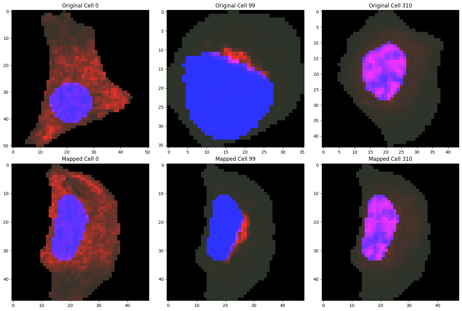
To assess whether the mapping parameters are appropriate, we can visualize examples of the localization patterns after mapping to the anchor cell.
[11]:
cells_to_plot = [0, 99, 310]
fig, axes = plt.subplots(2, len(cells_to_plot), figsize=(15, 10))

for idx, i in enumerate(cells_to_plot):
    # Plotting original cell
    plot_cell_image(cell_objects[i], channels=['nucleus', 'protein'], ax=axes[0, idx])
    axes[0, idx].set_title(f'Original Cell {i}')

    # Plotting mapped cell
    mapped_cell_object = cell_objects[target_cell_ind].copy()
    for j, channel in enumerate(channels_to_map):
        mapped_cell_object.intensities[channel] = mapped_distbs[j][i]
    plot_cell_image(mapped_cell_object, channels=['nucleus', 'protein'], ax=axes[1, idx])
    axes[1, idx].set_title(f'Mapped Cell {i}')

plt.tight_layout()
plt.show()
After mapping all cells to the anchor cell, we compute pairwise Wasserstein distances between the mapped protein distributions to quantify differences in subcellular localization. As in the morphology analysis, we can cluster cells based on these localization distances to identify groups with similar protein localization patterns and use UMAP to visualize the resulting space in two dimensions.
[12]:
ot_dmats = gw_mapped_ot_pairwise_parallel(cell_objects[target_cell_ind], mapped_distbs, num_processes=cpu_count(), chunksize=20)
Computing pairwise OT distances:
100%|██████████| 69378/69378 [41:01<00:00, 28.18it/s]
[13]:
# Compute UMAP representation of the OT localization space
reducer = umap.UMAP(metric="precomputed", random_state=1)
embedding = reducer.fit_transform(ot_dmats[0])

# Cluster cells based on the OT localization space using the leiden algorithm
ot_clusters = cajal.utilities.leiden_clustering(ot_dmats[0], resolution=0.005, seed=1)

# Visualize the OT localization space
plotly.express.scatter(x=embedding[:,0],
                       y=embedding[:,1],
                       template="simple_white",
                       hover_name=["cell_" + str(i) for i in range(ot_dmats[0].shape[0])],
                       color = [str(c) for c in ot_clusters]
                       )
/opt/conda/lib/python3.12/site-packages/umap/umap_.py:1865: UserWarning:

using precomputed metric; inverse_transform will be unavailable

/opt/conda/lib/python3.12/site-packages/umap/umap_.py:1952: UserWarning:

n_jobs value 1 overridden to 1 by setting random_state. Use no seed for parallelism.
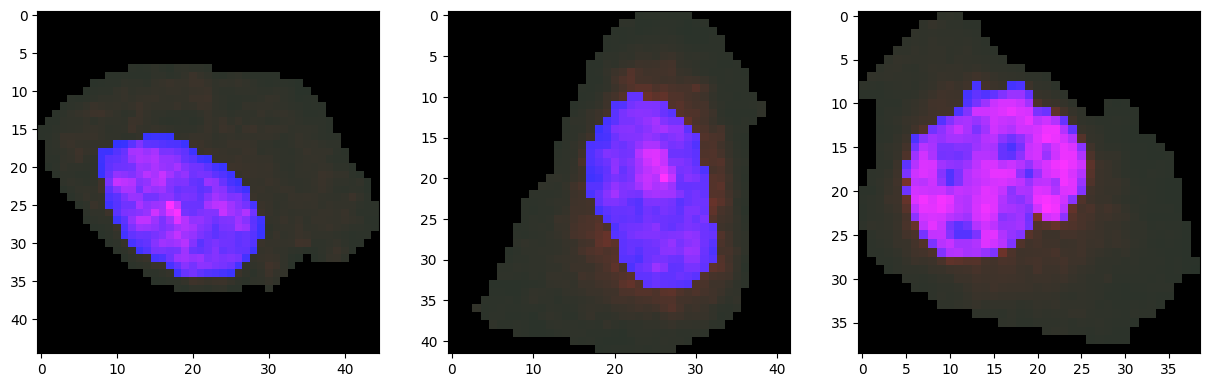
We can visualize representative cells from cluster 0 together with their protein distributions.
[14]:
cells_to_plot = [335, 270, 309] # Example cells from cluster 0
fig, axes = plt.subplots(1, len(cells_to_plot), figsize=(15, 5))
for ax, i in zip(axes, cells_to_plot):
    plot_cell_image(cell_objects[i], channels=['nucleus', 'protein'], ax=ax)
plt.show()
We can also color the UMAP representation of the optimal transport localization space by the localization pattern annotations from the Human Protein Atlas. As expected, the annotated localization patterns separate in the localization space.
[15]:
plotly.express.scatter(x=embedding[:,0],
                       y=embedding[:,1],
                       template="simple_white",
                       hover_name=np.array(["cell_" + str(i) for i in range(ot_dmats[0].shape[0])]),
                       color = np.array([str(c) for c in cell_metadata['locations']])
                       )
Applying existing cell image analysis methods to mapped cells
CellAligner-OT uses optimal transport distances to quantify differences in subcellular protein localization after mapping each cell to the anchor-cell morphology. However, mapped cells can also be used as input to existing cell image analysis methods, such as CellProfiler, Cytoself, or Paired Cell Inpainting. For downstream analysis with external tools, we can export the mapped cells as individual images.
[ ]:
output_dir = '/workspaces/CellAligner/mapped_cell_images'  # Path to save mapped cell images (the folder must already exist)
cell_image_channels = ['nucleus', 'protein']
for i in range(len(cell_objects)):
    # Create a cell object for the mapped cell
    mapped_cell_object = cell_objects[target_cell_ind].copy()
    for j, channel in enumerate(channels_to_map):
        mapped_cell_object.intensities[channel] = mapped_distbs[j][i]
    # Generate cell image from mapped cell object
    mapped_cell_image = make_cell_image(mapped_cell_object, channels=cell_image_channels)
    # Write mapped cell image to file
    ski.io.imsave(os.path.join(output_dir, f'mapped_cell_image_{i}.tif'), mapped_cell_image)
The make_cell_image function generates multi-channel images. The first channel contains the cell segmentation mask, and the remaining channels correspond to the entries specified by the channels parameter.
Using multiple anchor cells
One characteristic of CellAligner is that localization analysis after anchor-cell mapping can depend on the choice of anchor cell. In practice, we have found that choosing the centroid cell in the GW morphology space often produces informative localization analyses. However, users may want their analysis to be more robust to the choice of anchor cell.
To address this, we suggest mapping the protein distributions of each cell to multiple anchor cells and integrating the resulting localization spaces. One natural way to select anchor cells is to first cluster the GW morphology space and then choose the centroid cell from each morphological cluster. This approach uses a broad range of cellular morphologies when constructing the localization spaces.
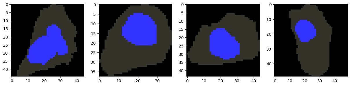
Here, we use CellAligner-OT to construct a separate localization space for each anchor cell. Note that, because this approach repeats the GW-based mapping and optimal transport computations for each anchor cell, it can substantially increase the runtime of the analysis.
[19]:
# Find centroid cell for each GW morphology cluster
cluster_centroids = []
for c in np.unique(gw_clusters):
    cluster_inds = np.where(gw_clusters == c)[0]
    # subset the GW distance matrix to only the cells in the cluster
    gw_dmat_cluster = gw_dmat[np.ix_(cluster_inds, cluster_inds)]
    # find the centroid cell in the cluster
    cluster_centroid_idx = find_centroid(gw_dmat_cluster)
    cluster_centroid = cluster_inds[cluster_centroid_idx]
    cluster_centroids.append(cluster_centroid)

# Visualize centroid cells for each GW morphology cluster
fig, axes = plt.subplots(1, len(cluster_centroids), figsize=(15, 5))
for ax, i in zip(axes, cluster_centroids):
    plot_cell_image(cell_objects[i], channels=['nucleus'], ax=ax)
plt.show()
[20]:
centroid_mapped_distbs = []
centroid_ot_dmats = []
for target_cell_ind in cluster_centroids[1:]:
    # Mapping all cells to anchor cell
    mapped_distbs = map_to_anchor_cell(cell_objects,
                                        channels_to_map,
                                        target_cell_ind, # cell to map to
                                        method='fused', # 'fused' for full mapping, 'fused' for partial mapping
                                        fused_channel='nucleus', # addition info to consider for mapping
                                        fused_cost=1000, fused_param=0.1, # controls weight of additional info
                                        compartment_specific=True) # parallelization parameters
    # Compute OT distance matrix for the mapped protein distributions
    ot_dmats = gw_mapped_ot_pairwise_parallel(cell_objects[target_cell_ind], mapped_distbs, num_processes=cpu_count(), chunksize=20)
    centroid_mapped_distbs.append(mapped_distbs)
    centroid_ot_dmats.append(ot_dmats)

    out_dir = '/workspaces/CellAligner/mapped_distances'  # Path to save distance matrices (the folder must already exist)
    for target_cell_ind, mapped_distbs, ot_dmats in zip(cluster_centroids, centroid_mapped_distbs, centroid_ot_dmats):
        with open(os.path.join(out_dir, f'anchor_{target_cell_ind}_mapped_distbs.pickle'), 'wb') as f:
            pickle.dump(mapped_distbs, f, protocol=pickle.HIGHEST_PROTOCOL)
        with open(os.path.join(out_dir, f'anchor_{target_cell_ind}_ot_dmats.pickle'), 'wb') as f:
            pickle.dump(ot_dmats, f, protocol=pickle.HIGHEST_PROTOCOL)
Mapping cells to target cell:
100%|██████████| 373/373 [1:32:34<00:00, 14.89s/it]
Computing pairwise OT distances:
100%|██████████| 69378/69378 [41:37<00:00, 27.78it/s]
Mapping cells to target cell:
100%|██████████| 373/373 [1:31:14<00:00, 14.68s/it]
Computing pairwise OT distances:
100%|██████████| 69378/69378 [39:04<00:00, 29.59it/s]
Mapping cells to target cell:
100%|██████████| 373/373 [1:20:07<00:00, 12.89s/it]
Computing pairwise OT distances:
100%|██████████| 69378/69378 [40:30<00:00, 28.54it/s]
Having computed a subcellular localization space based on each cluster centroid, we now build a consolidated space that integrates information across the individual localization spaces. We do this using the Weighted Nearest Neighbors (WNN) algorithm introduced in:
Hao, Y. et al. Integrated analysis of multimodal single-cell data. Cell 184, 3573–3587 (2021).
We first construct one Modality object for each localization space. The cajal.wnn.wnn() function then takes a list of Modality objects, together with the number of nearest neighbors to consider in each space.
[22]:
import cajal.wnn

# Extract protein OT dmat from each centroid cell
centroid_protein_ot_modalities = [cajal.wnn.Modality.of_dmat(ot_dmats[0]) for ot_dmats in centroid_ot_dmats]
# Integrate OT localization spaces from each centroid cell using WNN
integrated_space = 1-cajal.wnn.wnn(centroid_protein_ot_modalities, k=5)
The Weighted Nearest Neighbors algorithm returns an asymmetric similarity matrix. For visualization with UMAP, we symmetrize the matrix before embedding the consolidated representation in two dimensions.
[23]:
def symmetrize(a):
    a = a.copy()
    a[a == 0] = np.max(a)
    b = a + a.T
    b = np.minimum(a,b)
    b = np.minimum(b,a.T)
    d=np.zeros(a.shape[0],dtype=int)
    b[d,d]=0
    return np.array(b)

wnn_dmat = symmetrize(integrated_space)

# Compute UMAP representation of the OT localization space
reducer = umap.UMAP(metric="precomputed", random_state=1)
embedding = reducer.fit_transform(wnn_dmat)

# Visualize the OT localization space
plotly.express.scatter(x=embedding[:,0],
                       y=embedding[:,1],
                       template="simple_white",
                       hover_name=["cell_" + str(i) for i in range(wnn_dmat.shape[0])],
                       color = [str(c) for c in cell_metadata['locations']]
                       )